Do you have a problem with noisy data obtained from your accelerometer sensor? Learn how to remove noise from accelerometer in short practical example. You will understand digital filtering and learn how to make your measurements smoother.
Digital Filters
In general, we distinguish two kinds of digital filters FIR (filters with Finite Impulse Response ) and IIR (recurrence filters with Infinite Impulse Response). FIR filters are easier to implement so we try to use them first. If you would like to learn more about other filter design let me know in the comment section.
FIR filter
Filtering with an FIR filter is quite easy to understand. All it comes to a sliding window through raw data and calculating the subsequent output values, so filtering with FIR is similar to the moving average. Length of the sliding window is called filter order. The first four steps of the filtering process are illustrated in the picture below. Vector filed with a’s contains raw data and vector with c’s contains coefficients. Finally, y’s are subsequent values of the filter output. Easy right? 🙂
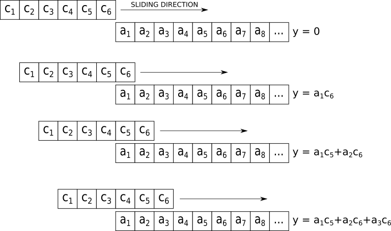
From a programmer’s point of view, the whole process can be done with two nested loops. The first one for moving through coefficient vector and the second for raw data vector.
The tricky part of a design process is the calculation of coefficients. The math behind that is not straightforward and it will be omitted here. (But if you would like to read about that let us know in the comments section.) Don’t worry, you don’t have to know all the math to learn how to design digital filters. We will use the Octave or MATLAB tools for calculating coefficients, removing the noise from the data and much more. Let’s see how to do this!
Practical example

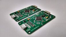
In this example, we will design a filter for removing high-frequency noise and bias caused by Earth’s gravity. The data was collected by the external USB accelerometer mounted on vibrating aluminum rod with a sampling frequency set to 3200 Hz (samples per second) and acceleration range was set to ±4 g. Z-axis was parallel to Earth’s gravity, so this is the reason the data is biased. A plot of the collected data during the first five seconds is bellow
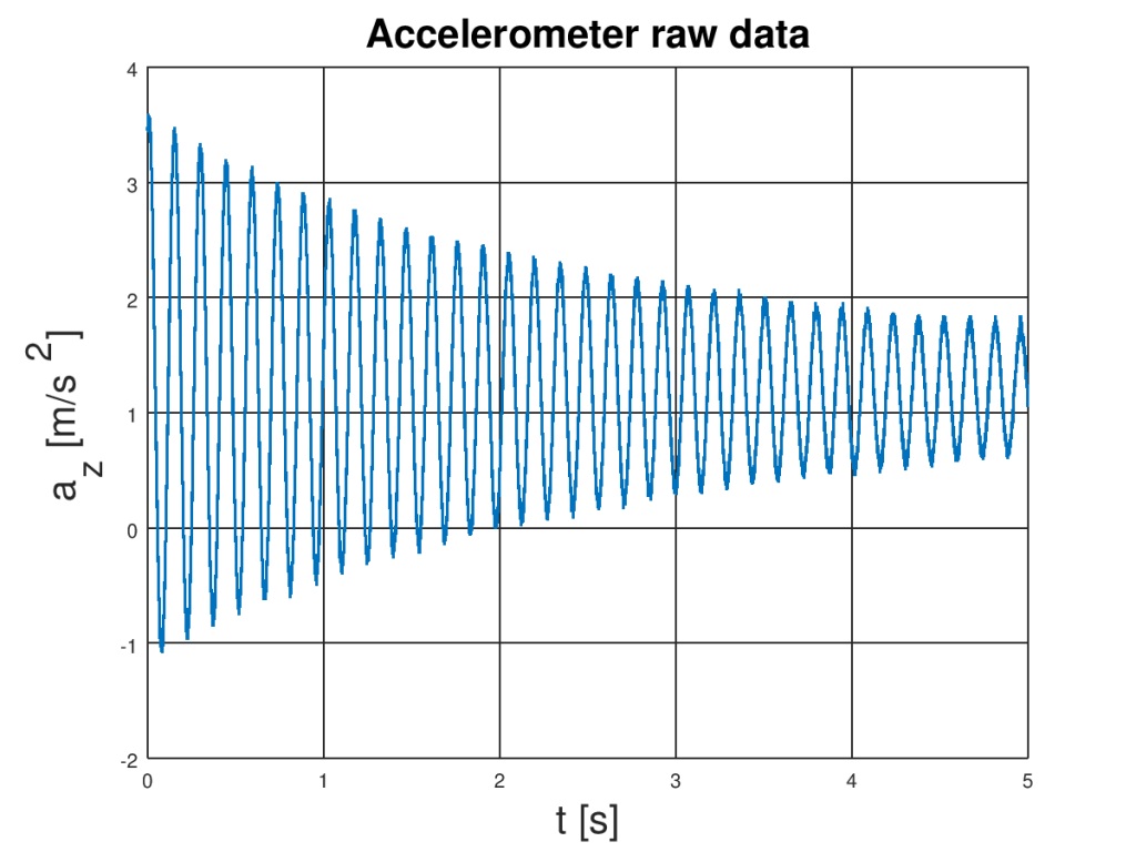
You can easily see that oscillations are shifted by around 1 g. The accelerometer noise can be visible especially in the local maxima and minima. Both DC component and noise can be filtered out from our signal because they have different spectra than oscillations of the rod. To obtain resonance frequency of the rod it is a good idea to look on the signal spectrum. Here it is:
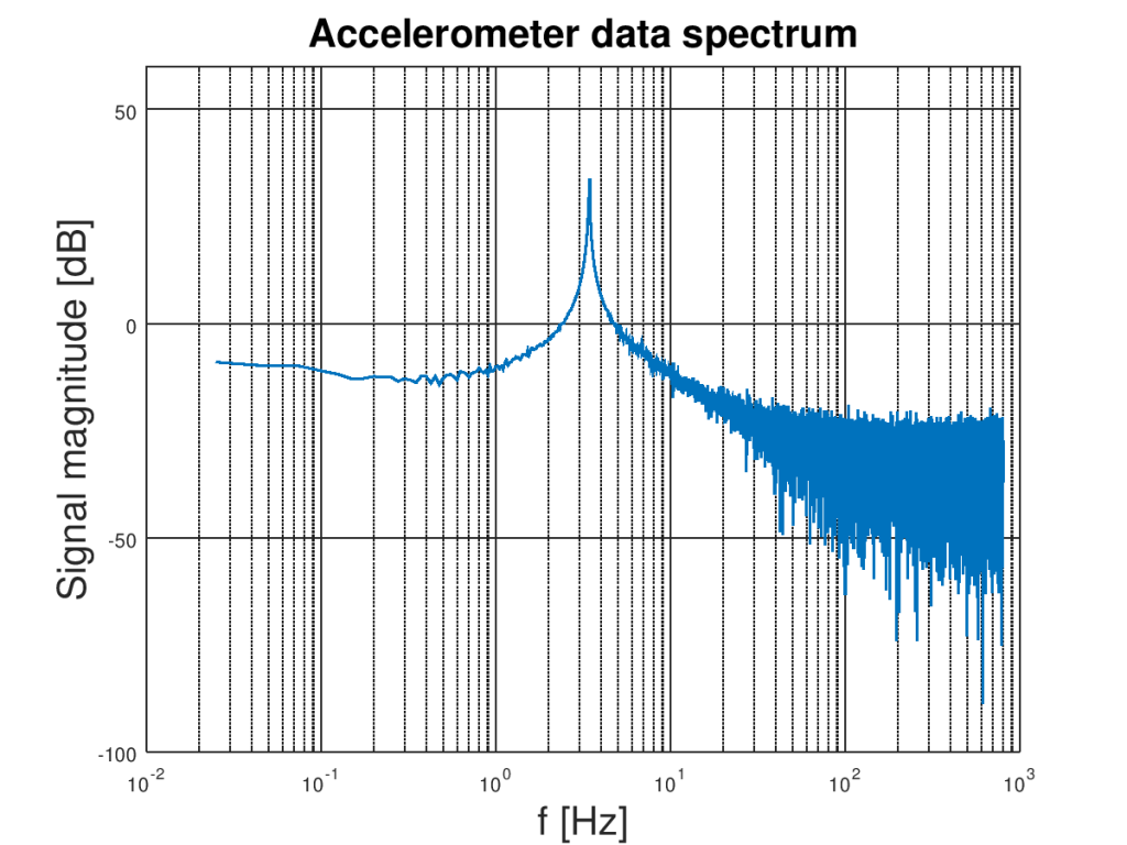
The zero-frequency component (bias) is not visible here because of the logarithmic plot. Anyway, its spectral amplitude is huge compared to rest. The natural frequency oscillation spectrum can be found between 3.0 Hz and 10 Hz so we need a bandpass filter that passes that range and cutoff anything else. Let’s design it using Octave. The script should work in MATLAB too. Necessary code is on the listing bellow
% Sampling frequency
fs = 3200;

% Nyquist frequency
fn = fs/2;

% Band pass filter frequencies [Hz]
fa =  3.0;
fb =  10.0;

% Normalized frequencies
fa_n = fa / fn;
fb_n = fb / fn;

% Calculate filter coefficients
% Attenuation (dB)
A = 40;
% Bandwidth
BW = fb-fa;
N = 2/3 * log10(1/(delta1 * delta2)) * fs/BW

filter_order = 1829;
c = fir1(filter_order, [fa_n, fb_n], "pass");
freqz(c,1, 5000, fs)
In the beginning, sampling and Nyquist frequencies are defined. We have to define filter cutoff frequencies and normalize them. To do so they have to be divided by the Nyquist frequency. Keep in mind that cutoff frequency doesn’t mean that the signal will be dumped to zero outside the passing region of filter. It actually means that it will be attenuated by 3 dB (which means that in the signal units it will be square root of 2 smaller) at these points and decrease further away.
To fully specify the FIR signal filter we need to assume the filter order. Let’s use the following approximated formula for this

N is the filter order. Delta one is a ripple in passband and delta two is a ripple in the stopband. BW is a bandwidth (in our case is 10 Hz – 3 Hz = 7 Hz). Let’s say that we want a filter that has ripples delta1 = 10^-4 in the passband and delta2 = 10^-2 in the stopband. After simple calculation, we get that filter order should be around 1829 taps. It’s quite a big number of taps but that is because of narrow bandwidth.
Now all these numbers i.e. filter order and normalized cutoff frequencies can be used for calculation of filter coefficients using following Octave / MATLAB code
c = fir1(filter_order, [fa_n, fb_n], "pass");
freqz(c,1, 5000, fs)
The first function calculates FIR filter coefficients and freqz plots characteristic of the filter. The second argument of the freqz is used in the case of IRR filters and should be set to 1 for FIR filters. The third argument specifies the number of points in the plot and the last argument is sampling frequency used for setting real values of the frequency axes. You can find frequency and phase characteristic on plots bellow.
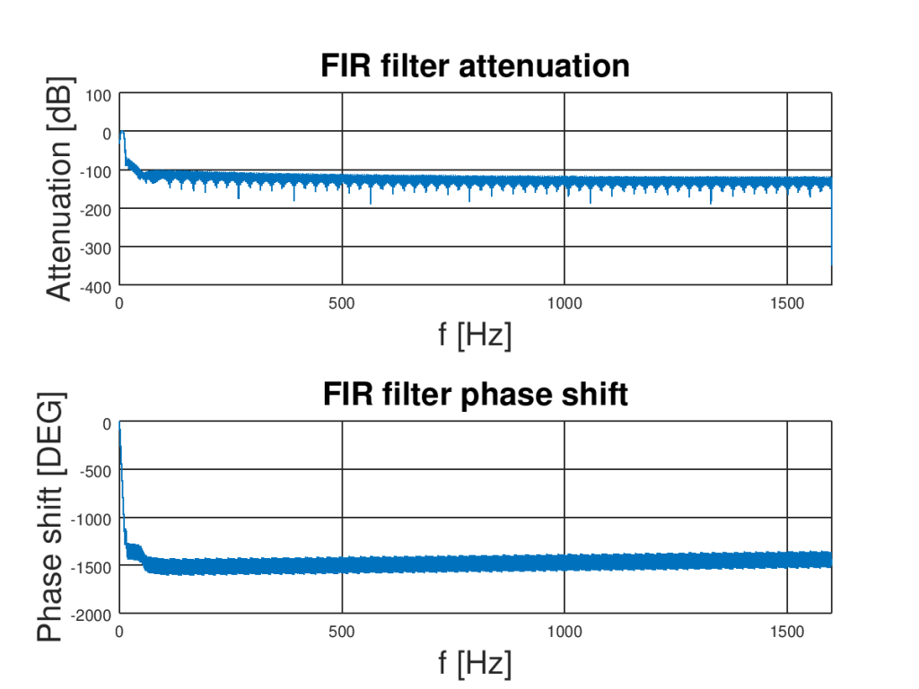
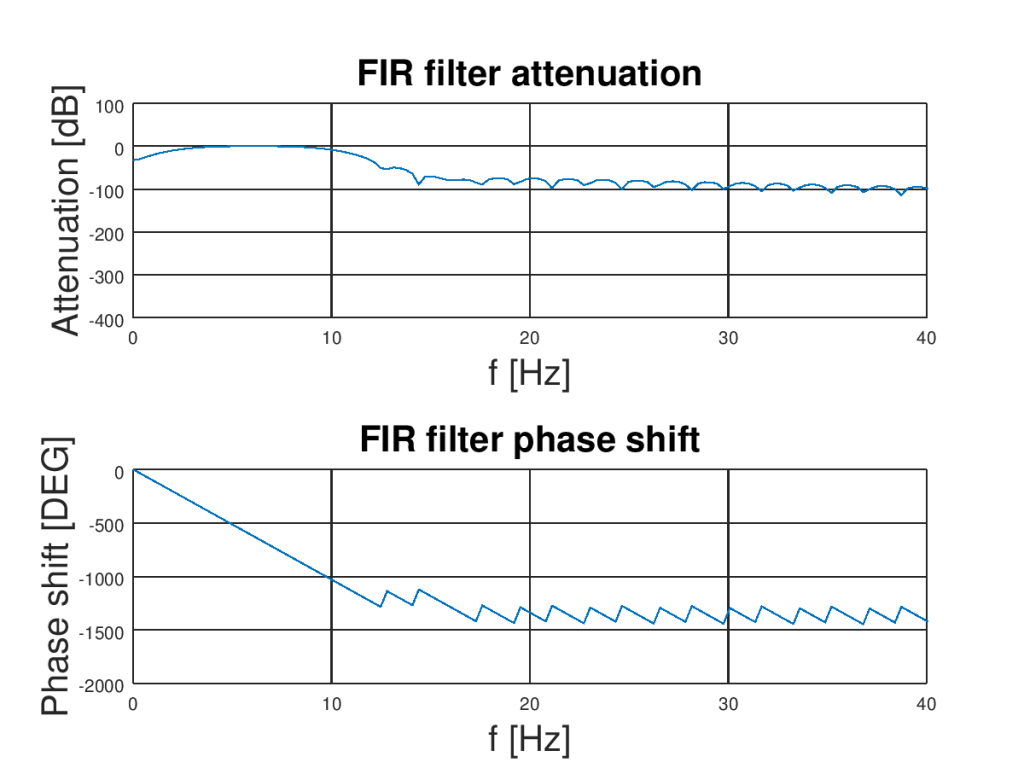
You can clearly see that we constructed a digital filter. As was noticed before it has cutoff frequencies at 3 Hz and 10 Hz (amplitude is attenuated by 3 dB in those points). The nice thing about FIR filters is that they have linear phase behavior in the passing region. It is good because components with different frequencies obtain the same delay and signal will not be distorted in this region.
Results
Okay, we have designed filter so finally let’s use it for its purpose! Here is the code used for actual applying
% Applay filter
y = filter(c, 1, az);
We have to use “filter” function for that. I take calculated earlier coefficients and produces output data vector thought ‘sliding’. The result is plotted bellow
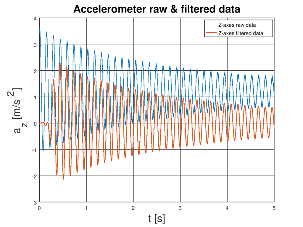
You can clearly see that bias is removed! Good job! But wait… how about high-frequency noise? Of course, I can tell you that it is removed because plot it much smoother but don’t believe me so easy let’s see it on the spectrogram of the filtered signal. Here it is

Looks much better than the last one especially at frequencies higher than the natural frequency of the rod. Most of the high-frequency noise is dumped bellow -50 dB! That is very good! That is what we wanted 🙂
Conclusions
We have learned the basics of FIR filters and apply them to a real problem. You can find the whole code HERE. Try to understand and modify the Octave code it will help you learn much more.
Share your thoughts and questions in the comment section to help others!


2 Comments
Pedja · September 9, 2019 at 8:27 pm
Great info.
Can something similar be applied to simpler data source, like piezo element as vibration detector? I tried to use piezo element to detect tapping, but i was not fully successful filtering noise.
Dariusz · September 9, 2019 at 8:47 pm
Thank you Pedja! 🙂
I think so, especially if the taping signal is much stronger than noise (above noise level).
In this case, you don’t need bandpass filter like in this example but only high pass filter (taping should have strong high frequency component).
To be sure I would try to record a signal with and without taping and check algorithm on PC then implement it in the source code.